Heroku App Link: https://precipitation-ml.herokuapp.com/
Note for Heroku app: Heroku free tier is being used. Give some time for Heroku dyno to come out of sleep if opening the link after a while.
GitHub Repository
See the link below for the code used to get the DataFrame used in this research. https://github.com/singparvi/Global-Precipitation/blob/master/Data_and_Code/Get_Precipiration_Data_NASA.ipynb
The code for the predictive modelling done in this project can be found in the link:- https://github.com/singparvi/Global-Precipitation/blob/master/Data_and_Code/Predict_Precipitation.ipynb
Abstract
Climate is becoming increasingly unpredictable over decades and it has never been more critical to make a better prediction on climate in human history. There is a substantial human and capital cost involved with a severe climate event. Current meteorological models can predict the climate in any area of the world with great accuracy. This research aims at predicting Precipitation using historical information and leveraging Multiple Linear Regression (MLR) in python Machine Learning to make a prediction. The prediction does not have to be for the following week or month, but it can be many years in the future. Multiple models were run using weather data from NASA and at best, an R^2 of 48.5% was obtained. The R^2 value may seem low but the Mean Absolute Error (MAE) has a 67% improvement from the baseline. The low R^2 was attributed to the non-availability of crucial climate information that could be added later to make a more refined prediction. Temperature was identified as the key feature in predicting Precipitation. This research’s best model’s predictions may enable decision-makers like governments or even insurance companies (with financial interests) to make predictions to plan for policies or undertaken risks.
Finding the Data and the JSON hurdle
Finding the data itself was a big hurdle in this project. The data must provide a learning opportunity and at the same time, Machine Learning practices can be applied on it. The data must have enough observations to devote time to. At least 100,000 so that there are enough observations to train, validate and then test. On the other hand, the data must relate to something that can tie into a business case.
After much investigation, it was finalized to take up the topic first to predict Rainfall. Precipitation was the only thing that was closest to the topic of interest.
NASA maintains an app called POWER Single Point Data Access 1 that provides data in JavaScript Object Notation (JSON) format through an Application Programming Interface (API) to users based on the geographical location of interest. NASA’s POWER app requires latitude and longitude to provide the weather information. The latitude and longitude of various countries were gathered using an existing CSV file from GitHub user albertyw 2.
A program was written in python notebook that takes in the latitude longitude information from the country list, pass it to NASA’s app to fetch the following information:-
- Lattitude (degrees in decimal)
- Longitude (degrees in decimal)
- Elevation (m)
- PRECTOT - Precipitation (mm day-1)
- QV2M - Specific Humidity at 2 Meters (g/kg)
- PS - Surface Pressure (kPa)
- TS - Earth Skin Temperature (C)
- T2MDEW - Dew/Frost Point at 2 Meters (C)
- T2M - Temperature Range at 2 Meters (C)
- WS50M - Wind Speed at 50 Meters (m/s)
- WS10M - Wind Speed at 10 Meters (m/s)
- T2MWET - Wet Bulb Temperature at 2 Meters (C)
- T2M_RANGE - Temperature Range at 2 Meters (C)
- RH2M - Relative Humidity at 2 Meters (%)
- KT - Insolation Clearness Index (dimensionless)
- CLRSKY_SFC_SW_DWN - Clear Sky Insolation Incident on a Horizontal Surface (kW-hr/m^2/day)
- ALLSKY_SFC_SW_DWN - All Sky Insolation Incident on a Horizontal Surface (kW-hr/m^2/day)
- ALLSKY_SFC_LW_DWN - Downward Thermal Infrared (Longwave) Radiative Flux (kW-hr/m^2/day)
The python code also merges the country code, latitude and longitude data to make a single data frame for use. The data included weather data for each day for 240 countries from 1980 to 2020. The resulting dataset had 3506400 rows × 22 columns.
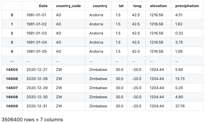 NASA-POWER-DataFrame
The data frame built was used in the research further. The learning to now be able to use JSON data available publically, send JSON requests, receive and interpret and convert them to pandas DataFrame was a small achievement in the machine learning model.
EDA and Machine Learning Model
Data from NASA’s application was cleaned and unnecessary or repetitive columns were dropped. Before getting into features and target selection, another feature was included in the data that should affect the Precipitation of any interest area. Based on a hypothesis that Precipitation will be higher in countries with more forest areas, Forest Area data from World Bank 3 was imported in the data frame as a feature through pandas merge function.
Due to resource limitations and quick turnarounds in model training, only the last twenty years of data were considered.
The data was ready for some Exploratory Data Analysis (EDA). Pandas Profiling was used to generate a report to see the type of data, missing values and data distribution.
The features were selected to be the following:-
- country_code
- lat
- long
- elevation
- surface_pressure
- skin_temperature
- dew_frost
- temperature2m
- windspeed10m
- windspeed50m
- wet_bulb_temp
- temp_range
- clearness_index
- clear_sky_insolation
- all_sky_insolation
- radiative_flux
- Forest_Cover(sq km)
The definition of all the features mentioned above was provided in the text above. Precipitation was chosen as the target.
The target was skewed to the right due to the presence of some 300 observations.
Baseline
Precipitation mean was chosen to set a baseline to compare the model performance. Precipitation mean was calculated for the entire data and was determined as 2.787 mm. Mean Absolute Error (MAE) was calculated and was found to be 3.379 mm. The baseline MAE is used to compare various models to see how each model fare in precipitation predictions.
Models
The model pipelines that use more time and resources in fitting the data frame from 2001 - 2020 was split as follows:-
Train - Data from 2008 - 2012 Validate - Data from 2013 only Test - Data from 2014
The various models run and their findings are discussed below:-
1. Ordinal Encoder and RandomForestRegressor pipeline
The code to instantiate and fit the pipeline was as simple as:-
1
2
3
4
5
pipeline_randomforest_OE = make_pipeline(
    ce.OrdinalEncoder(),
    RandomForestRegressor(n_estimators=100, random_state=42, verbose=1,n_jobs=-1)
)
pipeline_randomforest_OE.fit(X_train, y_train)
Since the data was super clean with no missing values, compute or scaling were not used.
Parameters to benchmark the model:-
| Parameter | Value |
|---|---|
| Time to fit the model | 22 sec |
| Training Score (R2) | 93.70 % |
| Validation Score (R2) | 44.02 % |
| Test Score (R2) | 44.22 % |
| Baseline MAE | 3.379 mm |
| Model MAE | 2.198 mm |
| Improvement over Baseline MAE | 53.73 % |
2. OneHotEncoder and RandomForestRegressor pipeline
The code to instantiate and fit the pipeline was:-
1
2
3
4
5
pipeline_randomforest_OHE = make_pipeline(
    ce.OneHotEncoder(use_cat_names=True),
    RandomForestRegressor(n_estimators=100, random_state=42, verbose=1,n_jobs=-1)
)
pipeline_randomforest_OHE.fit(X_train, y_train)
Parameters to benchmark the model:-
| Parameter | Value |
|---|---|
| Time to fit the model | 222 sec |
| Training Score (R2) | 93.70 % |
| Validation Score (R2) | 47.76 % |
| Validation Score (R2) | 47.30 % |
| Baseline MAE | 3.379 mm |
| Model MAE | 1.965 mm |
| Improvement over Baseline MAE | 71.89 % |
3. OrdinalEncoder and XGBoost pipeline
Before the XGBoost pipeline can be instantiated and fit, train, validation and test dataset were updated as follows:-
Train - Data from 2001 - 2012 Validate - Data from 2013 - 2016 Test - Data from 2017 - 2020
This was done as XGBoost is able to fit the model much faster as compared with the RandomForestRegressor.
The rest was similar to what was done in the past. The code to instantiated and fit the pipeline was:-
1
2
3
4
5
pipeline_xgboost = make_pipeline(
    ce.OrdinalEncoder(),
    XGBRegressor(n_estimators=100, random_state=42, verbose=1, n_jobs=-1)
)
pipeline_xgboost.fit(X_train, y_train)
Parameters to benchmark the model:-
| Parameter | Value |
|---|---|
| Time to fit the model | 11.47 sec |
| Training Score (R2) | 59.00 % |
| Validation Score (R2) | 48.45 % |
| Test Score (R2) | 35.98 % |
| Baseline MAE | 3.379 mm |
| Model MAE | 2.022 mm |
| Improvement over Baseline MAE | 67.09 % |
Analysis
Some correction in Model MAE was expected as RandomForestRegressor tries to fit a model with infinite depth. The model score for the RandomForestRegressor reflects this while the model wasn’t doing very well with the validation score. Another thing to note in the XGBoost model is that the data for a longer duration was used compared to the earlier run models. This may be another source due to which our improvement over the baseline was reduced compared to the previous model.
Features Importances from XGBRegressor
XGBRegressor was used to extract the top 15 features that contribute to the prediction of Precipitation.
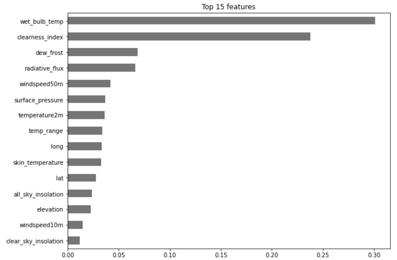 Top 15 Features as determined after XGBRegressor Run
Permutation Importance from XGBRegressor
Permutation importance provides an insight in ranking the features of the data by permuting different values in any feature. Web bulb temperature still ranks the top in predicting the Precipitation, however, the ranking has changed for other factors, as shown in the output below.
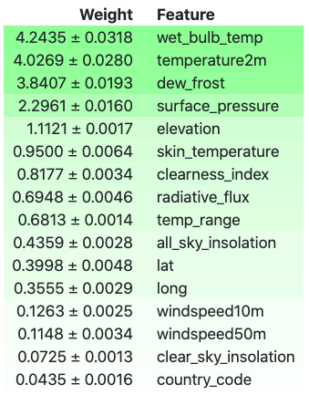 Image Showing Permutation Importance by priority
Partial Dependence Plot (PDP)
A Partial Dependence Plot was built to see the effect of more than one feature on the predicted Precipitation. From the PDP, it can be inferred that the relationship between the features and the target is monotonic.
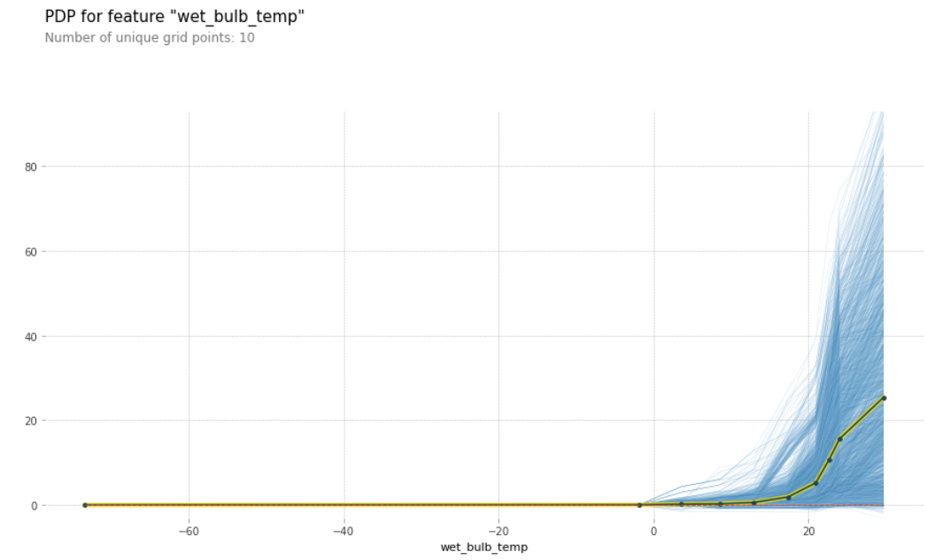 Partial Dependence Plot showing the Variation of Precipitation with Wet Bulb Temperature
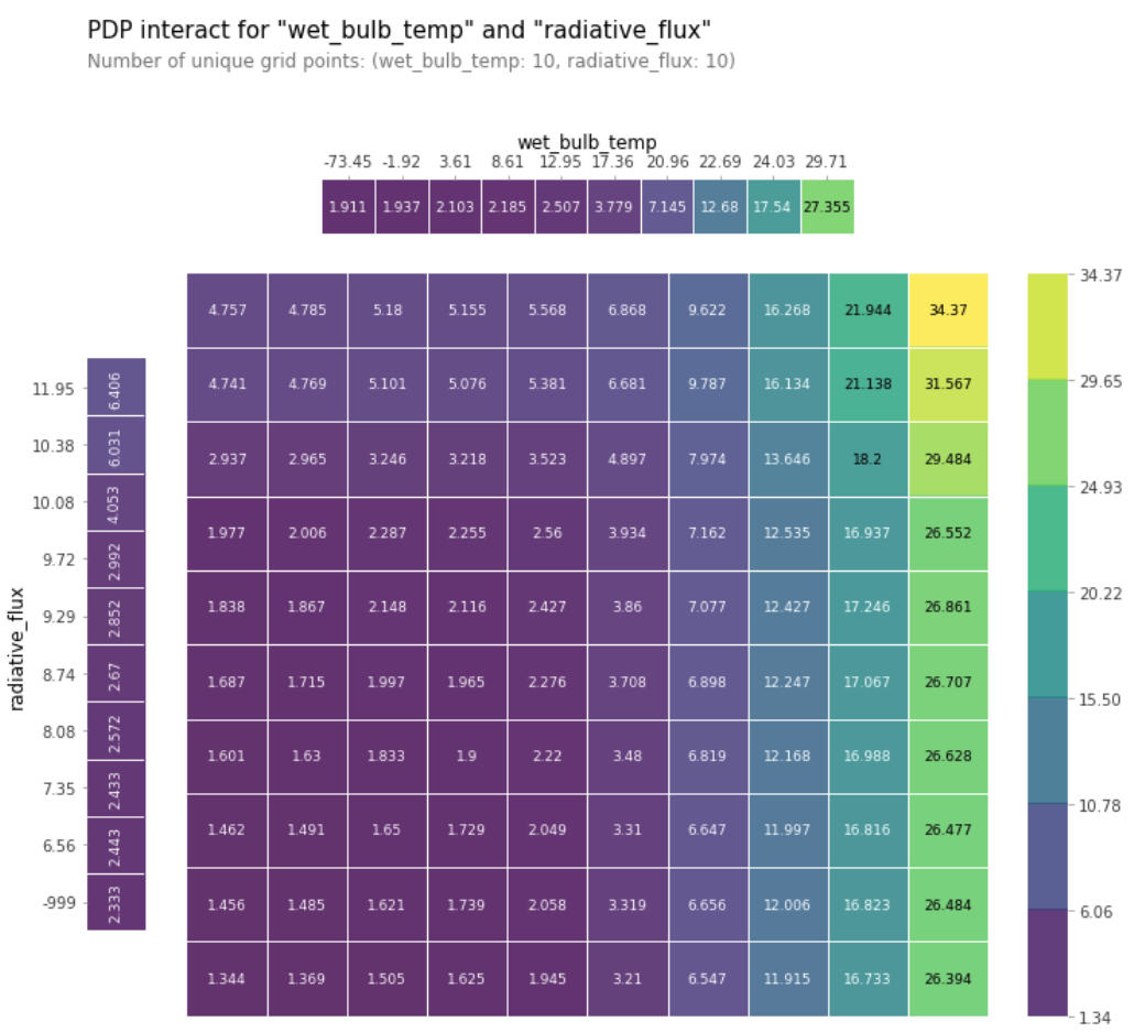 Partial Dependence Plot showing the Variation of Precipitation with Wet Bulb Temperature and Radiative Flux
Shap Values
Shap values are what the features contribute to the final predicted value.
 Image Showing how Precipitation Changes with Change in Features
Conclusion
Based on all the features used in this research, Temperature was the key feature that predicts Precipitation of any region. With temperatures rising globally due to global warming, the research in this project shows that the precipitation levels are also likely to increase. If it interests you in testing the XGBoost model to make predictions, then use the app in the link below.